Researchers' Zone:
Here is how an algorithm is baking optimal brownies and discovering drugs
A new scientific paradigm revolving around the use of algorithms is solving optimisation problems and increasing scientists’ efficiency – and you can try it at home!
What do cutting-edge scientific approaches to drug discovery and chocolate brownies have in common?
Well, more than you might think!
We all have been in situations where we are faced with different ways of solving a problem that directly impact the time spent and the quality of the outcome.
For instance, imagine you are mining for gold. How do you determine at what depth to search?
Or maybe you want to bake the best brownie possible, then the amount of each ingredient, oven temperature and the baking time are important input features.
From these two examples, we can conceptualize tasks with a clear objective which depends on input features (mining depth or recipe for cake). These kinds of so-called ‘optimisation problems’ are numerous in science and engineering, and it is often of great interest to optimise objectives like reduced time consumption, increased profit or quality.
A new game-changing paradigm of how to solve optimisation problems is emerging in science.
In this article you will learn what, how and why that is, as well as how this new paradigm could help you in your day-to-day life.
A new scientific paradigm – scientists out?
Optimisation can be achieved via many different approaches.
Commonly, we can apply experience, scientific domain knowledge and intuition in combination with explicit mathematical models to improve the outcomes of a given problem. However, while this human-driven approach has yielded many great results in science and engineering, it suffers from inherent flaws:
Firstly, the need for generalization and simplification. In scientific models, the world is described using concepts with some degree of generalization as a consequence of the difficulty of dealing with the daunting complexity of the world.
This simplification often relies on assumptions that are only partly true and thus might prevent important correlations from being discovered.
Secondly, the basis in human experience might lead to personal biases, like preferring certain methods because of tradition or personal interests, which might be suboptimal for some problems.
The problem of human bias and assumptions has been shown in competitions between scientific experts and machine learning predicting interplay between proteins and has even been used to generate scientific hypotheses for battery manufacturing.
Great job! Can you please repeat that 196 times?
While computers and humans have different upsides when designing experiments, robots and computers are definitely better when it comes to structured, repetitive tasks both in terms of speed and stamina.
A scientist must go home from work at some point, and once they have optimised the problem somewhat, they are inclined to stop and be satisfied with the result, missing potential improvements.
These drawbacks are among the reasons that a new paradigm in the approach to scientific discovery is arising.
The combination of two rapidly developing scientific fields has enabled this approach.
Firstly, automation of scientific experiments, meaning that experiments can be run in ‘high throughput’ and can controlled from a computer.
Secondly, the advances in modelling our world using machine learning algorithms.
Combining these capabilities allows for a setup that is not only fully automated but also adaptively learning. These approaches are gaining traction because they circumvent the problems with the human expert approach.
Therefore, these new approaches have the potential to push beyond human cognition, be immensely labour-saving and do repetitive tasks you can’t expect a human to do.
Thus, they potentially yield better results while simultaneously augmenting a human scientist to reach a desired target (be it a qualitative or a quantitative target) faster.
Closed-loop optimisation – humans go drink coffee!
That is all very good, but what is an efficient way to carry this out?
One example of using an automated data-driven approach to solving scientific problems is found in the concept of ‘Closed-loop Bayesian Optimization’.
Let's save the ‘Bayesian’ part and start by uncovering the idea of Closed-loop Optimization.
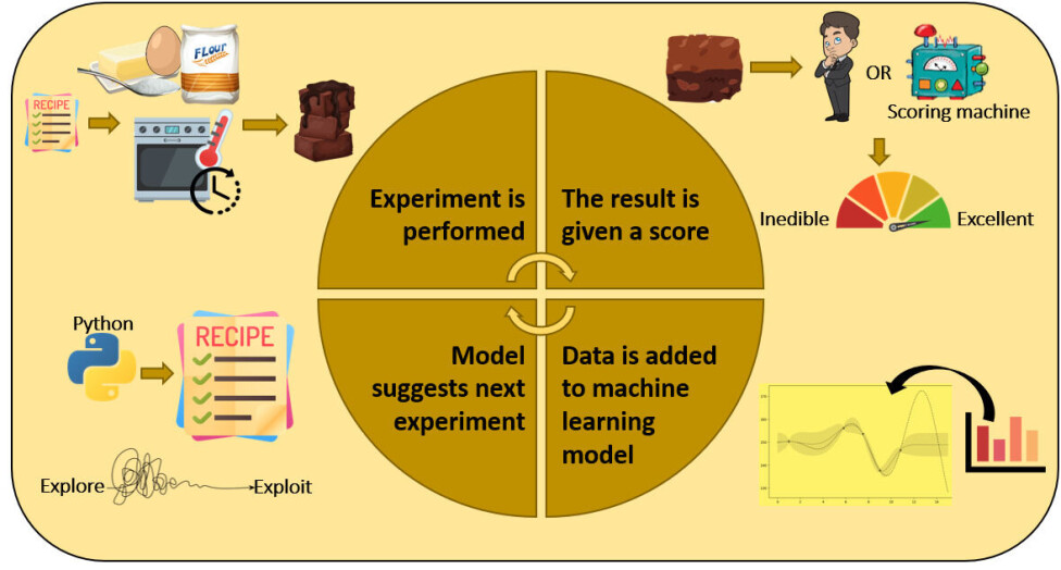
Firstly, you perform some initial experiments to shed light on the effect of the preselected features (think flour, sugar etc. in the brownie-example).
Next you measure some outputs and give a score (based on what you want to achieve).
Finally, you use this information to design the next experiment to be tried. All of this is done without human intervention – it cycles in a ‘closed’ loop.
A black box function
The problem to be optimised is often referred to as a »black box function« because it takes several input features (think the amounts of ingredients and oven settings) and returns an output value (a brownie), which can be evaluated to give a score.
The function is a »black box« because it cannot easily be represented by mathematic expressions, but nonetheless, the output depends on the input features.
The loop is further explained in figure 1 taking the chocolate brownie as example.
Remember that this is only truly closed loop, if the baking and scoring (tasting) can also be done automatically.
Real-world examples – stem cells, online shopping and drones
As you might have guessed, optimisation in closed loop is an effective strategy, which is why it is being applied to a multitude of problems including optimisation of electric car charging, sales on webpages, differentiation of stem cells, drone-flying and many more.
Interestingly, the optimisation of these very different problems is solved by essentially the same algorithm!
Closed-loop optimisation has been implemented at Novo Nordisk A/S in the optimisation of chemical reactions, to help discover new therapeutics.
Here the ‘ingredients of the brownie’ are chemicals in the reaction, and the oven is a ‘pipetting robot’ (an automated device that moves small amounts of liquid) performing the reactions.
Reactions, where the desired product is colourful are especially well suited for closed loop optimization, as the intensity of the product-colour can be easily measured as a metric of success.
The optimisation runs entirely without human intervention, and the algorithm comes increasingly closer to an optimal recipe for the reaction.
But how does the algorithm decide what the next experiment should be?
(How) Does the algorithm think?
Spoiler alert: the algorithm doesn’t ‘think’.
Instead, it is a machine learning algorithm that uses a clever implementation of statistics.
Let's lay out conceptually how the algorithm works without knocking anyone over with formulas.
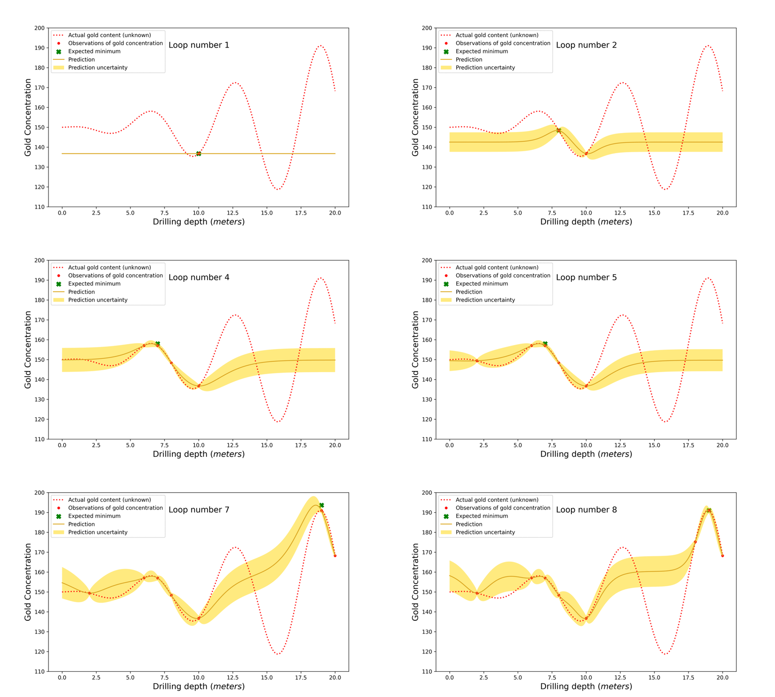
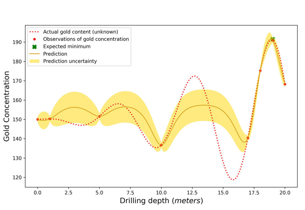
Imagine an optimisation in gold mining with one input feature; the depth of mining, and one score; the concentration of gold (think grams of gold per ton of dirt).
As seen in figure 2 below, there exists a function describing the relationship between input and output (shown in red dashed), but this function would be unknown to us in the real world.
We have observed the gold concentration at several depths, shown by the red points. Based on these points, the Bayesian optimisation algorithm predicts a function of the expected gold amount at all depths (gold line) and how uncertain this prediction is (gold shaded area).
This modelling is done using two assumptions:
firstly, that the gold concentration is similar at two depths that are also similar, such that if you know the gold concentration at one depth, you have information about the concentration at a similar depth.
Secondly, that the function describing the gold concentration is smooth with round turns.
Exploitation and exploration
Now to the magic: To predict at what depth to mine at order to find the most gold, the algorithm looks at two things.
Firstly, where is the expected value highest? And secondly, where are we most uncertain (large gold shaded area) about the expected gold concentration (because it is favourable to explore that territory).
Searching where the expected value is high is called exploitation (of current knowledge) and searching in areas of uncertainty is called exploration.
We need the exploration since the prediction can be very wrong in areas of high uncertainty, as seen around x = 12.5 in figure 2.
Whether the model is mostly exploitive or exploratory is tuned by the scientist, and this can be very important for the outcome of the optimisation.
In the gif in figure 3 you see how the search for gold using Bayesian optimisation works.
Figure 3: The step-by-step process of Bayesian optimisation. First the model searches in the middle of the search space (0-20 m) at 10 m. Then, based on the prediction and uncertainty, the algorithm decides where to search next. The algorithm first finds a local maximum but luckily explores unknown territory in loop number 6. Observe how ‘loop number’ 7 finds the best possible depth. This is only known because the actual gold content is plotted for illustrative purposes. However, in a real-life scenario, this target would be unknown, and one would just need to decide at what stage the best suggested value is good enough.
Cutting edge optimisation tool
The ability of optimising problems in a closed loop using algorithms carries great potential in science. The algorithm ‘thinks’ differently than a human experimenter and the robots can work around the clock.
For some optimisations, the Bayesian optimisation approach has been shown to outcompete scientific experts.
But the interesting thing to note here is not the competition. It is how automation and algorithms are starting to augment scientists in well-defined tasks freeing their time for more complex tasks that humans excel at.
In addition, Bayesian optimisation is an interesting example of a new scientific approach to gaining insight using a limited amount of data from processes with many independent features (like the long list of potential combinations of ingredients in a cake).
The coupling between carefully designed experiments and advanced data analysis compares favourably to traditional one factor at a time hypothesis testing in science.
This article was originally published on our Danish sister site, Forskerzonen.
References:
- Timothy Patrick Jenkins' profile (DTU)
- James Love's profile (ResearchGate)
- Søren Bertelsen's profile (ResearchGate)
- 'Bayesian reaction optimization as a tool for chemical synthesis', Nature (2021), DOI: 10.1038/s41586-021-03213-y
- 'Closed-loop optimization of fast-charging protocols for batteries with machine learning', Nature (2020), DOI: 10.1038/s41586-020-1994-5
- 'Robotic Search for Optimal Cell Culture in Regenerative Medicine', bioRxiv (2020), DOI: 10.1101/2020.11.25.392936
